OLAP (Online Analytical Processing)

Online Analytical Processing (OLAP) is a computer technology used to quickly analyze large volumes of multi-dimensional historical data from multiple perspectives. It powers business intelligence, budgeting, forecasting, and complex reporting by enabling fast queries across massive datasets without slowing down daily transactional systems.

Key OLAP Operations

• Roll-up: Summarize data by moving up a concept hierarchy (e.g., daily sales to monthly sales).
• Drill-down: Move from summary data down to detailed data (e.g., yearly sales down to specific days).
• Slice: Isolate a single dimension from a data structure to create a specific sub-view.
• Dice: Select specific values across multiple dimensions to analyze a focused subset.
• Pivot: Rotate the axes of a data view to see relationships from a new angle.

OLAP vs. OLTP Comparison

• OLAP (Online Analytical Processing): Optimized for complex read-heavy analytical queries, historical tracking, and large aggregations across billions of rows using columnar storage. Examples include Snowflake, Google BigQuery, and ClickHouse.
• OLTP (Online Transaction Processing): Optimized for real-time, high-concurrency operational tasks like fast individual row inserts, updates, and daily customer transactions. Examples include MySQL and PostgreSQL.

source: AI overview

OLAP (Online Analytical Processing) is the technology behind many Business Intelligence (BI) applications. OLAP is a powerful technology for data discovery, including capabilities for limitless report viewing, complex analytical calculations, and predictive “what if” scenario (budget, forecast) planning.

Unlike relational databases, OLAP tools do not store individual transaction records in two-dimensional, row-by-column format, like a worksheet, but instead use multidimensional database structures—known as Cubes in OLAP terminology—to store arrays of consolidated information. The data and formulas are stored in an optimized multidimensional database, while views of the data are created on demand.

source: https://olap.com/olap-definition/

Parquet files and Delta Lake

Column-based format - files are organized by column, rather than by row, which saves storage space and speeds up analytics queries.

Apache Parquet is implemented using the record-shredding and assembly algorithm, which accommodates the complex data structures that can be used to store the data. Parquet is optimized to work with complex data in bulk and features different ways for efficient data compression and encoding types.

Parquet and Delta Lake

The open source Delta Lake project builds upon and extends the Parquet format, adding additional functionality like ACID transactions on cloud object storage, time travel, schema evolution, and simple DML commands (CREATE/UPDATE/INSERT/DELETE/MERGE). Delta Lake implements many of these important features through the use of an ordered transaction log that makes data warehousing functionality possible on cloud object storage.

source: https://www.databricks.com/blog/what-is-parquet

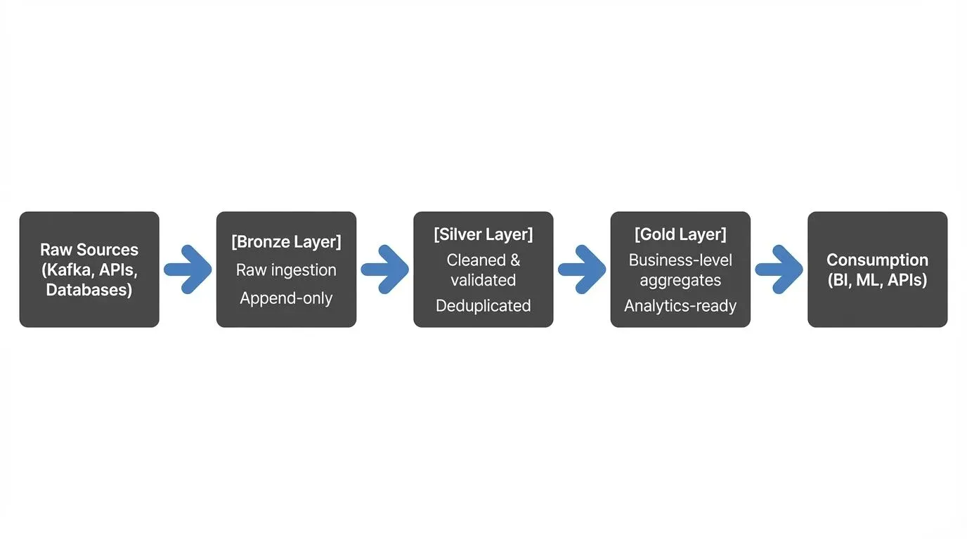
Medallion architecture: bronze, silver, and gold

 A layered data organization system:

• Bronze: Raw, unprocessed data as it arrives from source systems. Preserves original state for auditing and reprocessing.
• Silver: Cleaned, deduplicated, and standardized data. Conforms to consistent naming and formatting conventions across the organization.
• Gold: Business-ready, curated datasets optimized for analytics and reporting. This is where data becomes actionable for business users.

This three-tier structure moves data from its raw form through progressive refinement, improving quality and usability at each stage.

See related TWOTW: ETL - extract, translate, load

Sources:

• Medallion Architecture: Bronze, Silver & Gold Layers Explained (2026 Guide)
• Data Lake Zones: Bronze, Silver, Gold Architecture | Conduktor
• Understanding the Three Layers of Medallion Architecture

Simpson's Paradox

Simpson's Paradox is a statistical phenomenon that occurs when you combine subgroups into one group. The process of aggregating data can cause the apparent direction and strength of the relationship between two variables to change.

source: https://statisticsbyjim.com/basics/simpsons-paradox/

source: https://www.tjanesky.com/post/simpsons-paradox

See the TWOTW articles on clustering.

Benford's Law

Benford’s law describes the relative frequency distribution for leading digits of numbers in datasets. Leading digits with smaller values occur more frequently than larger values. This law states that approximately 30% of numbers start with a 1 while less than 5% start with a 9. According to this law, leading 1s appear 6.5 times as often as leading 9s! Benford’s law is also known as the First Digit Law.

If leading digits 1 – 9 had an equal probability, they’d each occur 11.1% of the time. However, that is not true in many datasets. The graph displays the distribution of leading digits according to Benford’s law.

Analysis of datasets shows that many follow Benford’s law. For example, analysts have found that stock prices, population numbers, death rates, sports statistics, financial and tax information, and billing amounts often have leading digits that follow this distribution. 

Uses for Benford’s Law

Analysts have used it extensively to look for fraud and manipulation in financial records, tax returns, applications, and decision-making documents. They compare the distribution of leading digits in these datasets to Benford’s law. When the leading digits don’t follow the distribution, it’s a red flag for fraud in some datasets.

When Does Benford’s Law Apply and Not Apply

Benford’s law generally applies to data that fit some of the following guidelines:

• Quantitative data.
• Data that are measured rather than assigned.
• Ranges over orders of magnitudes.
• Not artificially restricted by minimums or maximums.
• Mixed populations.
• Larger datasets are better.

Elaborations on Guidelines

Benford’s law often does not apply to assigned numbers, such as ID numbers, phone numbers, and zip codes.

It works best for data that range over multiple orders of magnitudes from very low to very high. You can cover the 10s, 100s, 1000s, and so on. For example, population and incomes can range from very low to very high.

Conversely, if the range of values is restricted, it affects the leading digits, and Benford’s law is less likely to apply. For example, human characteristics naturally fall into restricted ranges. Consequently, this distribution doesn’t apply to human ages, heights and weights. Similarly, limits imposed on potential values can also invalidate this law. Awards in small claims courts have an upper limit, which can negate Benford’s law.

Interestingly, mathematicians have proven that numbers from mixed populations follow Benford’s law. Mixed populations are things like all numbers pulled from a magazine issue. Obviously, those numbers will represent various topics and types of values. Benford himself did that with Reader’s Digest and newspapers. You can also combine data from different sources to achieve the same effect.

Like all distributions, larger datasets will produce observed relative frequencies that more closely approximate the theoretical values of Benford’s law. Smaller datasets can create relatively large deviations due to random error. Some analysts say datasets as small as 100 are acceptable, but most think a minimum size of 500 or even 1,000 is necessary.

Curiously, it will work in some cases where it should not. For example, it applies to house numbers even though those are assigned.

Benford’s Law Formula

Benford’s law formula is the following:

Where d = the values of the leading digits from 1 to 9.

The formula calculates the probability for each leading digit. The table below displays the probabilities that Benford’s law formula calculates for all digits.

Digit     Probability

1     30.1%

2     17.6%

3     12.5%

4     9.7%

5     7.9%

6     6.7%

7     5.8%

8     5.1%

9     4.6%

source: https://statisticsbyjim.com/probability/benfords-law/

Alarm Fatigue

Alarm fatigue or alert fatigue describes how busy workers become desensitized to safety alerts, and as a result ignore or fail to respond appropriately to such warnings. Alarm fatigue occurs in many fields, including construction and mining, healthcare, and the nuclear power field. Like crying wolf, such false alarms rob the critical alarms of the importance they deserve. Alarm management and policy are critical to prevent alarm fatigue. 

Examples

• Vehicle back-up alarms sound so frequently that they often become senseless background noise
• Electronic medical monitors tracking clinical information such as vital signs and blood glucose sound alarms so frequently, and often for such minor reasons, that they lose the urgency and attention-grabbing power which they are intended to have
• California Proposition 65 has been criticized for causing "over-warning" due to encouraging "meaningless warnings." There is no penalty for posting an unnecessary warning sign, and to the extent that warnings are vague or overused, they may not communicate much information to the end user. Many companies now routinely attach Prop 65 warning labels to any product of theirs that they think might possibly contain one of the 900 listed chemicals without testing to see whether the chemical is really present in their product and without reformulating their product, because it is cheaper to do so than to run the risk of being sued by Prop 65 enforcers.

Proposed solutions

• Identify by sound alone. Change alarm sounds to be softer and friendlier in order to improve identification of alarms. 
• Adjust the parameters and delays to alarms to match the traits and status. However, this directly trades sensitivity for specificity.
• Centrally monitor alarms where a trained person evaluates each alarm and distributes alerts only when necessary.
• Adjust automated alarm algorithms to be more specific and not overly sensitive to mitigate false alarms and balance sensitivity and specificity to still detect actionable conditions.

See also

• Alarm management – Usability factor in alarm systems
• Banner blindness – Tendency to ignore banner-size notices
• Compassion fatigue – Condition characterized by emotional and physical exhaustion
• False alarm – Deceptive or erroneous report of an emergency
• Habituation – Decrease in a behavioral response to a repeated stimulus
• Inattentional blindness – Condition of failing to see something in plain view
• Information overload – Decision making with too much information
• Normalization of deviance – Sociological phenomenon
• Semantic satiation – Psychological phenomenon

source: https://en.wikipedia.org/wiki/Alarm_fatigue

Braess's paradox

Braess's paradox is the observation that adding one or more roads to a road network can slow down overall traffic flow through it. The paradox was postulated in 1968 by German mathematician Dietrich Braess.

The paradox may have analogies in electrical power grids and biological systems. It has been suggested that in theory, the improvement of a malfunctioning network could be accomplished by removing certain parts of it. The paradox has been used to explain instances of improved traffic flow when existing major roads are closed.

The idea behind Braess's discovery is that the Nash equilibrium may not equate with the best overall flow through a network.

Adding extra capacity to a network when the moving entities selfishly choose their route can in some cases reduce overall performance. That is because the Nash equilibrium of such a system is not necessarily optimal. In a Nash equilibrium, drivers have no incentive to change their routes. While the system is not in a Nash equilibrium, individual drivers are able to improve their respective travel times by changing the routes they take. In the case of Braess's paradox, drivers will continue to switch until they reach Nash equilibrium despite the reduction in overall performance.

 

source: https://en.wikipedia.org/wiki/Braess%27s_paradox

analysis paralysis

Don’t Let Uncertainty Paralyze Your Decision-Making

When you’re living in a period of heightened uncertainty, your normal decision-making processes can break down. Some people become paralyzed and afraid to act, while others make quick decisions based on emotions or bias rather than facts. You can make careful, reasoned decisions by taking a strategic pause to stop and assess what information you have — and what you’re missing. First, identify what kind of data you’re working with and biases that might accompany it. For example, some data captures our attention because it's surprising, but we might overweigh it because it’s new or noteworthy. Next, identify which information matters most to your decision-making. There are an endless number of “known unknowns” out there, and exploring them all won’t help you. Instead ask yourself: What do I really need to know to move forward? Finally, formulate questions that will help you get the answers you need. Organize your questions into four categories — behavior, opinion, feeling, and knowledge — so that you bring both distance and a variety of perspectives to how you interpret the data. Following these practices will help you better address your emotional responses, name and confront them, and make more rational decisions in the face of uncertainty.

This tip is adapted from “How to Make Rational Decisions in the Face of Uncertainty,” by Cheryl Strauss Einhorn

KPI (key performance indicator)

Key performance indicators (KPIs) are metrics that organizations can use to track and target places to improve. Software teams should be able to tie each KPI to business initiatives or stated business values.

However, specific KPIs will vary from one project to another.

source: 14 top mobile app KPIs that advance development

Key performance indicators IT operations drive teams to work more efficiently -- but what drives KPIs?

"You have to accept this notion that what IT does has to be aligned with the outcomes of the business, not just with the weather inside the IT organization," said Joseph Pucciarelli, group vice president and IT executive advisor at IDC. 

As such, results-oriented metrics, such as those related to end-user and customer satisfaction, should replace, or at least supplement, some of the more traditional, process-focused IT metrics tied to time and cost.

A process-centric KPI for IT, for example, would be the rate at which help desk tickets are closed. This metric inspires speed in help desk technicians, but doesn't always satisfy users, especially if the issue isn't resolved correctly and they have to reopen a ticket. A more results-oriented KPI, in this example, would measure users' experience with the help desk ticket process.

source: Modern IT KPIs emphasize cloud, DevOps and user experience

Intelligent Communities Lifecycle (ICL)

The ICL is a relatively new technology platform for developing sustainable communities that was launched by the leading performance analysis solutions vendor, IES, last year. With the ICL, short for “Intelligent Communities Lifecycle,” IES has expanded its expertise to larger groups of buildings such as campuses and neighborhoods. The idea is the same—to apply sustainable design concepts—but now to entire communities and not just individual buildings.
This review explores the individual components of the ICL for modeling, monitoring, and analysis, and how they can be integrated into a digital twin into a digital twin for sustainable design.

source: http://www.aecbytes.com/review/2020/IES-ICL.html

optimal stopping

Having reached the 12th week of the process to hire a new employee, I recalled videos I had seen on how to know when to stop (see below). The examples are a bit simplified compared to hiring a real person, after all, the candidate must also decide when to stop looking for a job. Since either party can decline the relationship, the term "optimal" may not apply. Nevertheless, the optimal stopping theory does provide a good principle for how to establish a baseline of acceptability among the candidates. The theory works best with a known number of candidates or a limited amount of time to make the decision.

Optimal Stopping

Brian Christian, coauthor, with Tom Griffiths, of Algorithms to Live By. He writes, codes & lives in San Francisco. In an article on medium.com, he wrote:

If you want the best odds, spend 37% of your hunt noncommittally exploring options. You’re just calibrating. But after that point, be prepared to immediately commit  to the very first candidate you see that beats whatever you’ve already seen. This is not merely an intuitively satisfying compromise between looking and leaping. It is the provably optimal solution.

37% = 1/e

YouTube Videos

• When To Quit (According to Computer Science) (6:29)

Optimal Stopping. The Secretary Problem Explained. Taken from a chapter of the book "Algorithms to Live By - The Computer Science of Human Decisions" by Brian Christian and Tom Griffiths

• Mathematical Way to Choose a Toilet - Numberphile (7:49)

• The mathematics of love | Hannah Fry (TED Talk 17:00)

Bayesian _______

Bayesian _______

estimation

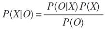
The problem is the quality of a 5 star rating depends not only on the average number of stars but also on the number of reviews. Bayesian estimation attempts to forgo computing a direct value from a limited number of observations and instead creates a probability distribution. It would seem clear that a 4.1-star rating with hundreds of reviewers has many that are happy. Therefore, it should probably appear before a 5-star rating with only one reviewer even though its average rating is lower. Bayes formula tells us how to compute the probability of X given O:

source: Computing a Bayesian Estimate of Star Rating Means

model

A Bayesian model can explicitly account for:

• Time. Perhaps old ratings should count for less than new ratings.
• Prior beliefs. Perhaps an unrated item from a bestselling author should appear above an unrated item from an unknown author.
• Attitudes toward risk. Exactly how risk-averse should the algorithm be about promoting items with a small number ratings?

source: Bayesian Average Ratings

trap

"The Bayesian Trap" Veritasium on YouTube. Bayes' theorem explained with examples and implications for life.

logic

Combine probabilistic logic and Bayesian networks to obtain the advantages of each in what is called Bayesian logic. Like probabilistic logic, it is a theoretically grounded way of representing and reasoning with uncertainty that uses only as much probabilistic information as one has, since it permits one to specify probabilities as intervals rather than precise values.

network

A Bayesian network is an augmented, directed acyclic graph, where each node corresponds to a random variable x and each edge indicates a direct influence among the random variables.

probability

Bayesian probability is an interpretation of the concept of probability, in which, instead of frequency or propensity of some phenomenon, probability is interpreted as reasonable expectation representing a state of knowledge or as quantification of a personal belief.

statistics

Bayesian statistics is a mathematical procedure that applies probabilities to statistical problems.

source: Bayesian Statistics explained to Beginners in Simple English

analysis

Bayesian analysis is a statistical paradigm that answers research questions about unknown parameters using probability statements. In Bayesian analysis, a parameter is summarized by an entire distribution of values instead of one fixed value as in classical frequentist analysis. Unique features of Bayesian analysis include an ability to incorporate prior information in the analysis, an intuitive interpretation of credible intervals as fixed ranges to which a parameter is known to belong with a prespecified probability, and an ability to assign an actual probability to any hypothesis of interest.

inference

Bayesian inference is a method of statistical inference in which Bayes' theorem is used to update the probability for a hypothesis as more evidence or information becomes available.

Bayes’ theorem

Bayes’ theorem describes the probability of an event, based on prior knowledge of conditions that might be related to the event. For example, if cancer is related to age, then, using Bayes’ theorem, a person’s age can be used to more accurately assess the probability that they have cancer, compared to the assessment of the probability of cancer made without knowledge of the person's age.

Named for Thomas Bayes, an English clergyman and mathematician, Bayesian logic is a branch of logic applied to decision making and inferential statistics that deals with probability inference: using the knowledge of prior events to predict future events.

State Flapping

Flapping occurs when a service or host changes state too frequently, resulting in a storm of problem and recovery notifications. Flapping can be indicative of configuration problems (e.g., thresholds set too low), troublesome services, or real network problems.

How exactly does one determine what "too frequently" means in regards to state changes for a particular host or service?

Whenever Nagios checks the status of a host or service, it will check to see if it has started or stopped flapping. It does this by:

• Storing the results of the last 21 checks of the host or service
• Analyzing the historical check results and determine where state changes/transitions occur
• Using the state transitions to determine a percent state change value (a measure of change) for the host or service
• Comparing the percent state change value against low and high flapping thresholds

A host or service is determined to have started flapping when its percent state change first exceeds a high flapping threshold.

A host or service is determined to have stopped flapping when its percent state goes below a low flapping threshold (assuming that it was previously flapping).

Let's describe in more detail how flap detection works with services...

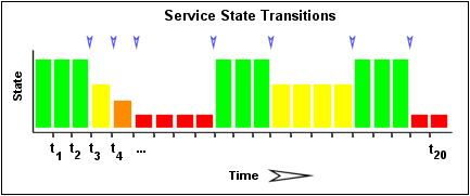
The image below shows a chronological history of service states from the most recent 21 service checks. OK states are shown in green, WARNING states in yellow, CRITICAL states in red, and UNKNOWN states in orange.

The historical service check results are examined to determine where state changes/transitions occur. State changes occur when an archived state is different from the archived state that immediately precedes it chronologically. Since we keep the results of the last 21 service checks in the array, there is a possibility of having at most 20 state changes. In this example there are 7 state changes, indicated by blue arrows in the image above.

The flap detection logic uses the state changes to determine an overall percent state change for the service. This is a measure of volatility/change for the service. Services that never change state will have a 0% state change value, while services that change state each time they're checked will have 100% state change. Most services will have a percent state change somewhere in between.

When calculating the percent state change for the service, the flap detection algorithm will give more weight to new state changes compare to older ones. Specifically, the flap detection routines are currently designed to make the newest possible state change carry 50% more weight than the oldest possible state change. The image below shows how recent state changes are given more weight than older state changes when calculating the overall or total percent state change for a particular service.

Using the images above, lets do a calculation of percent state change for the service. You will notice that there are a total of 7 state changes (at t₃, t₄, t₅, t₉, t₁₂, t₁₆, and t₁₉). Without any weighting of the state changes over time, this would give us a total state change of 35%:

(7 observed state changes / possible 20 state changes) * 100 = 35 %
 
Since the flap detection logic will give newer state changes a higher rate than older state changes, the actual calculated percent state change will be slightly less than 35% in this example. Let's say that the weighted percent of state change turned out to be 31%...

The calculated percent state change for the service (31%) will then be compared against flapping thresholds to see what should happen:

• If the service was not previously flapping and 31% is equal to or greater than the high flap threshold, Nagios considers the service to have just started flapping.
• If the service was previously flapping and 31% is less than the low flap threshold, Nagios considers the service to have just stopped flapping.

If neither of those two conditions are met, the flap detection logic won't do anything else with the service, since it is either not currently flapping or it is still flapping.

source: https://assets.nagios.com/downloads/nagioscore/docs/nagioscore/3/en/flapping.html